17 Pareto Distribution – Data Science with R

17.1 Introduction

Some patterns in life are surprisingly consistent. We’ve all noticed that a small number of people, products, or actions often account for a large share of the results, or outcomes. This idea is famously known as the Pareto effect or the 80/20 rule: roughly 80% of the outcomes come from 20% of the causes—and it shows up everywhere: in economics, business, social sciences, and even in nature. Respectively, the Pareto distribution is the statistical model behind this kind of pattern. It is a continuous distribution that helps us describe these seemingly imbalanced situations.

Named after the Italian economist Vilfredo Pareto who first observed that roughly 80% of land in Italy was owned by 20% of the population, this distribution helps us model situations with “heavy tails”. That means it accounts for the fact that extreme values, such as very rich individuals or very high-traffic websites are more common than we would expect from a normal distribution.

So, whenever we encounter a situation where a small proportion of items leads to a large proportion of outcomes or results, the Pareto distribution might be a good candidate for modeling it. In the sections that follow, we’ll explore what this distribution looks like, how it works mathematically, and how to simulate and visualize it in R. Along the way, we’ll see why it can be both powerful and tricky—especially since, in some cases, even the mean or the variance do not exist.

17.2 Where do we encounter the Pareto distribution?

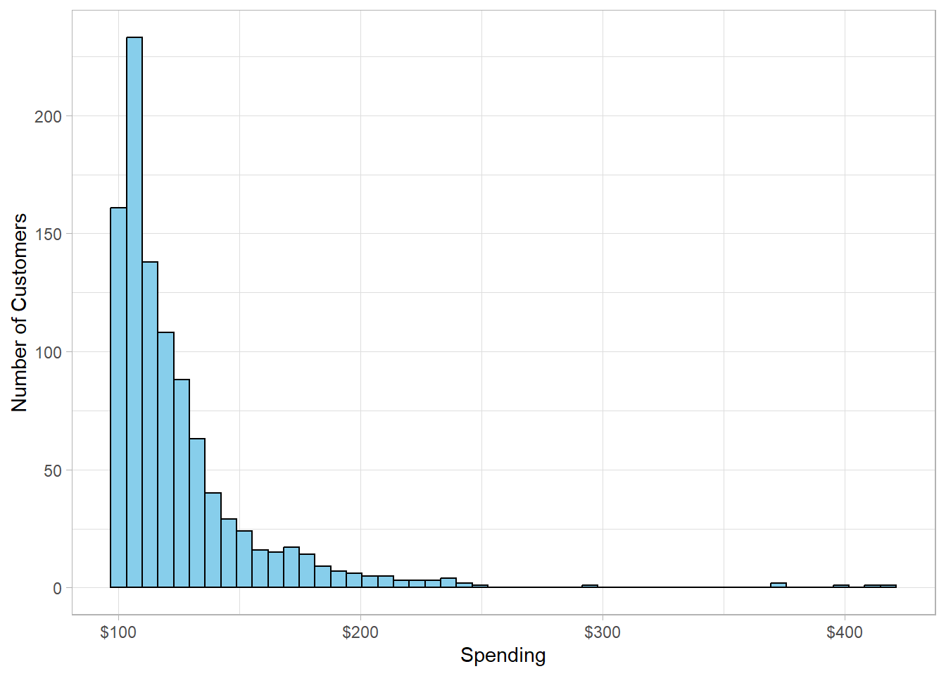
Imagine we run an online store and have data on how much each customer has spent over the past year. We can visualize this spending data as follows:

This distribution is right-skewed, meaning there are some extreme values on the right-hand side—customers who spend significantly more than the rest. What stands out is that a small percentage of customers account for a large share of total revenue. This is a classic example of the Pareto distribution in action, capturing situations where a few items (factors or persons) have a big impact, while most items contribute relatively little.

The Pareto distribution is encountered across many fields and contexts. In economics, it helps us visualize that income and wealth are often concentrated in the hands of a few individuals, highlighting patterns of economic inequality. In business, it guides us to focus on the small share of customers or products that generate the majority of profits or sales, allowing more effective allocation of marketing spend and operational resources. In ecology, it describes how a few species tend to dominate an ecosystem, while most species remain relatively rare. In computer science, the Pareto distribution appears in the distribution of file sizes, internet traffic, and system loads, where a small number of files or users account for the majority of activity. This wide range of applications shows how the Pareto distribution helps us make sense of many real-world phenomena characterized by imbalance and skewness.

17.3 What are the parameters and shape of the Pareto distribution?

The Pareto distribution is continuous, and has a probability density function as follows:

\[ f(x) = \frac{ax^{a}_{min}}{x^{a + 1}} \]

for \(x \ge x_{min}\) and \(a > 0\).

From the PDF, it is apparent that this distribution has two parameters: \(a\) and \(x_{min}\). The parameter alpha (\(a\)) is the shape parameter and controls how “heavy” the tail of the distribution is. A smaller alpha means the distribution is more skewed, with more extreme values occurring more often. As alpha increases, the distribution becomes less skewed and more concentrated near the minimum value. The parameter \(x_{min}\) is called scale and it is the minimum possible value that the random variable can take. As such, no values will be smaller than this cutoff.

The plot below shows three Pareto distributions, each with a different value of alpha but the same \(x_{min}\):

# Setting seed
set.seed(456)

# Create a data frame with 3 Pareto distributions
pareto_sim_1 <- tibble(Customer = 1:1000, Alpha = 1.5, Parameter = "a = 1.5")
pareto_sim_2 <- tibble(Customer = 1001:2000, Alpha = 3, Parameter = "a = 3")
pareto_sim_3 <- tibble(Customer = 2001:3000, Alpha = 10, Parameter = "a = 10")

# Join all data frames
pareto_sim <- pareto_sim_1 %>%
    bind_rows(pareto_sim_2,
              pareto_sim_3) %>%
    mutate(Spending = 100 / runif(n = Customer)^(1/Alpha))

# Plot the 3 distributions
pareto_sim %>% 
    ggplot(aes(x = Spending, 
               color = Parameter,
               group = Parameter)) +
    geom_density(linewidth = 1.5) +
    scale_x_log10() +
    labs(x = "Spending (log scale)", 
         y = "Density")

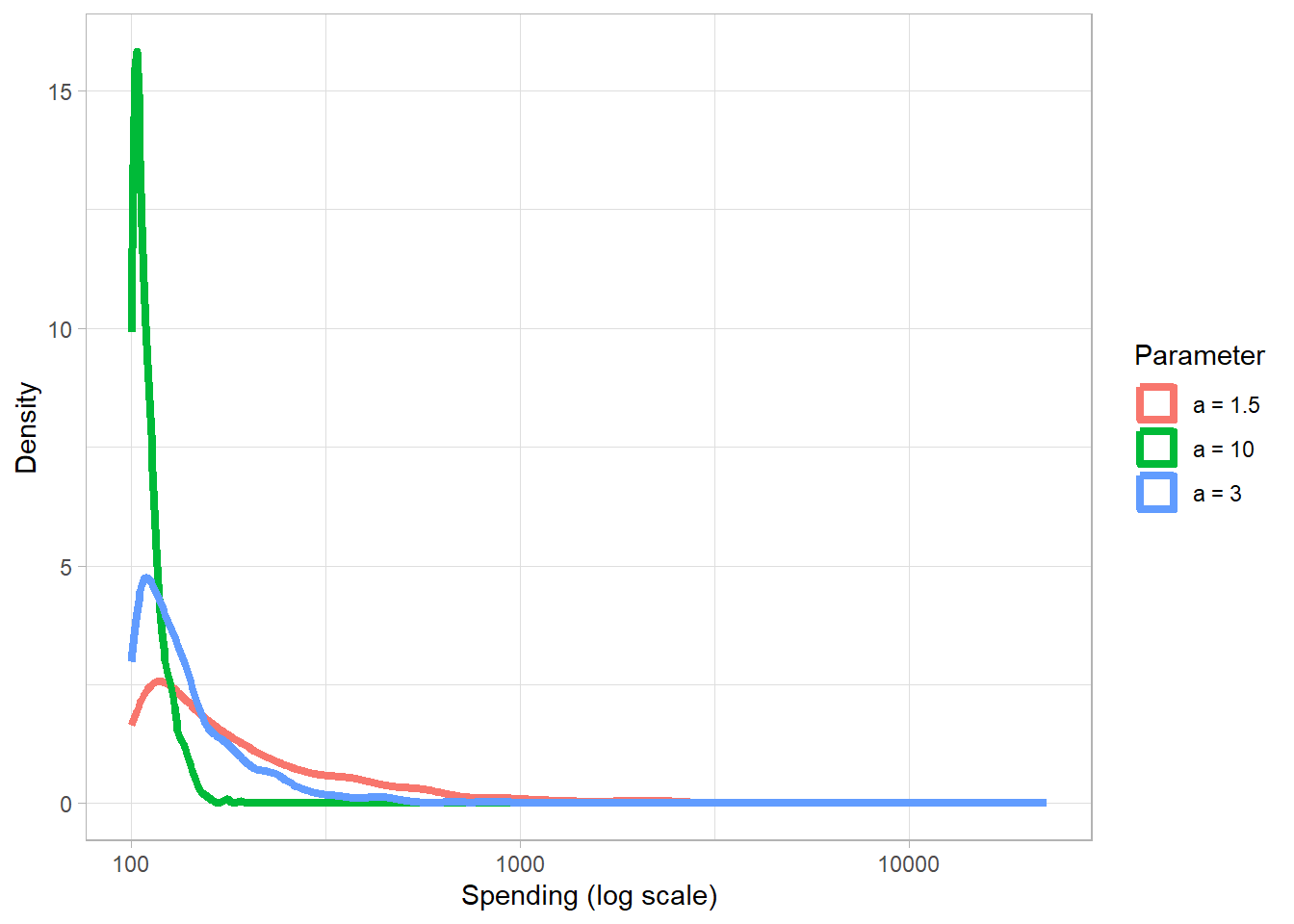
When \(a = 1.5\), the distribution has a very heavy tail, meaning larger values are encountered more frequently. When \(a = 3\), the tail is less heavy but still noticeable and finally when \(a = 10\), the tail is quite light, with large values becoming rare.

The expected value (or mean) of the Pareto distribution depends on both the shape (\(a\)) and the scale (\(x_{min}\)) parameters. Nonetheless, the mean exists only when \(a\) is greater than 1. Respectively, the variance exists only when \(a\) is greater than 2. Assuming that \(a\) is greater than 2, the expected value and the variance of the distribution can be calculated using the following formulas:

\[ E(X) = \frac{ax_{min}}{a - 1} \]

\[ Var(X) = (\frac{x_{min}}{a - 1})^2 \times \frac{a}{a - 2} \]

For example, if we set \(x_{min} = 100\) and \(a = 3\), then the mean of the variable \(X\) would be:

\[ E(X) = \frac{3 \times 100}{3 - 1} = 150 \]

At the same time, the variance would be:

\[ Var(X) = (\frac{100}{2})^2 \times \frac{3}{3 - 2} = 7500 \]

As we can see, both mean and variance exist in this case because \(a\) is greater than 2. When \(a\) is below 1 or 2, the denominator in these formulas becomes too small—or even zero—causing the mean or variance to diverge to infinity. This is a key feature of the Pareto distribution: depending on the value of \(a\), some of its moments may not exist. In practical terms, this means that averages and variability may become unreliable or undefined, which can make modeling, inference, or simulation results unstable or misleading—especially when extreme values dominate the data.

17.4 Calculating and Simulating in R

Unlike other common theoretical distributions, base R does not include built-in functions for the Pareto distribution. However, we can use the VGAM package, which provides a full set of functions for working with Pareto distributions. These functions follow a similar naming convention to base R distribution functions, like dnorm(), rbinom(), etc. Specifically:

dpareto() computes the density (PDF),
ppareto() gives the cumulative probability (CDF),
qpareto() returns quantiles, and
rpareto() generates random values.

Let’s simulate 10,000 observations from a Pareto distribution with shape parameter \(a = 10\) and minimum value \(x_{min} = 2000\):

# Libraries
library(tidyverse)
library(VGAM)

# Setting seed
set.seed(999)

# Simulate 10,000 values from a Pareto distribution
pareto_sim <- tibble(x = rpareto(n = 10000, scale = 2000, shape = 10))

# Plot the histogram
pareto_sim %>%
  ggplot(aes(x = x)) + 
  geom_histogram(fill = "skyblue", 
                 color = "black") +
  labs(x = "Simulated Values",
       y = "Count")

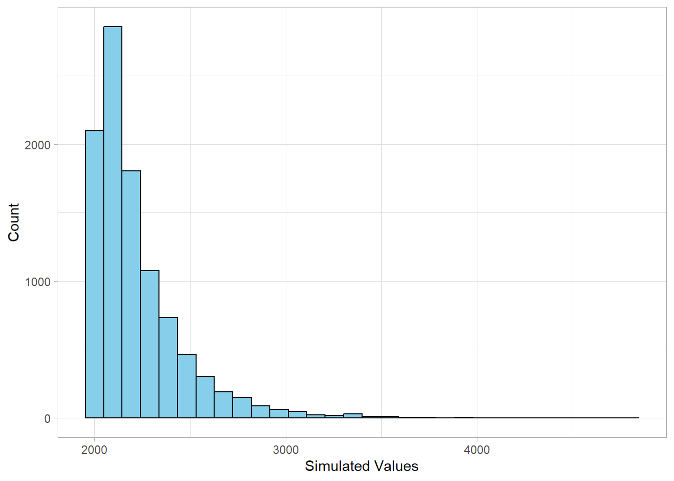
As expected, this distribution is right-skewed, with most values clustered near the minimum value (2000) and a few large values extending into the tail. Since the shape parameter is quite large (\(a\) = 10), the tail is relatively light, and extreme values would occur less frequently compared to smaller \(a\) values.

In addition to generating random numbers, we can calculate probabilities and quantiles using the other functions:

# Density at x = 2500
dpareto(2500, scale = 2000, shape = 10)

[1] 0.0004294967

# Probability of a value being less than or equal to 3000
ppareto(3000, scale = 2000, shape = 10)

[1] 0.9826585

# Quantile at the 95th percentile
qpareto(0.95, scale = 2000, shape = 10)

[1] 2698.566

These tools make it easy to explore the Pareto distribution through both simulation and analytical methods.

17.5 Recap

The Pareto distribution models situations where a small number of items account for a large share of the results—an idea often referred to as “the 80/20 rule”. It is commonly used in fields like economics, business, ecology, and computer science to describe imbalanced and heavy-tailed patterns.

This distribution is defined by two parameters and is known for its skewed shape, which can lead to undefined averages or variances depending on the parameter values. Using R, and specifically the VGAM package, we can simulate and explore the Pareto distribution through visualization and probability functions.